Trace - Format

The Format submenu defines how the measured data is presented in the graphical display.

The Format settings are closely related to the settings in the Scale submenu and in the Display menu. All of them have an influence on the way the analyzer presents data on the screen.

The analyzer allows arbitrary combinations of display formats and measured quantities (Trace – Measure). Nevertheless, in order to extract useful information from the data, it is important to select a display format which is appropriate to the analysis of a particular measured quantity; see Measured Quantities and Display Formats.

dB Mag

Selects a Cartesian diagram with a logarithmic scale of the vertical axis to display the magnitude of the complex measured quantity.

Properties: The stimulus variable appears on the horizontal axis, scaled linearly. The magnitude of the complex quantity C, i.e. |C| = sqrt ( Re(C)2 + Im(C)2 ), appears on the vertical axis, scaled in dB. The decibel conversion is calculated according to dB Mag(C) = 20 * log(|C|) dB.

Application: dB Mag is the default format for the complex, dimensionless S-parameters. The dB-scale is the natural scale for measurements related to power ratios (insertion loss, gain etc.).

The magnitude of each complex quantity can be displayed on a linear scale. It is possible to view the real and imaginary parts instead of the magnitude and phase. Both the magnitude and phase are displayed in the polar diagram.

Phase

Selects a Cartesian diagram with a linear vertical axis to display the phase of a complex measured quantity in the range between –180 degrees and +180 degrees.

Properties: The stimulus variable appears on the horizontal axis, scaled linearly. The phase of the complex quantity C, i.e. φ (C) = arctan ( Im(C) / Re(C) ), appears on the vertical axis. φ (C) is measured relative to the phase at the start of the sweep (reference phase = 0°). If φ (C) exceeds +180° the curve jumps by –360°; if it falls below –180°, the trace jumps by +360°. The result is a trace with a typical sawtooth shape. The alternative Phase Unwrapped format avoids this behavior.

Application: Phase measurements, e.g. phase distortion, deviation from linearity.

The magnitude of each complex quantity can be displayed on a linear scale or on a logarithmic scale. It is possible to view the real and imaginary parts instead of the magnitude and phase. Both the magnitude and phase are displayed in the polar diagram. As an alternative to direct phase measurements, the analyzer provides the derivative of the phase response for a frequency sweep (Delay).

Smith

Selects a Smith chart to display a complex quantity, primarily a reflection S-parameter.

Properties: The Smith chart is a circular diagram obtained by mapping the positive complex semi-plane into a unit circle. Points with the same resistance are located on circles, points with the same reactance produce arcs. If the measured quantity is a complex reflection coefficient (S11, S22 etc.), then the unit Smith chart represents the normalized impedance. In contrast to the polar diagram, the scaling of the diagram is not linear.

The axis for the sweep variable is lost in Smith charts but the marker functions easily provide the stimulus value of any measurement point. dB values for the magnitude and other conversions can be obtained by means of the Marker Format functions.

Polar

Selects a polar diagram to display a complex quantity, primarily an S-parameter or ratio.

Properties: The polar diagram shows the measured data (response values) in the complex plane with a horizontal real axis and a vertical imaginary axis. The magnitude of a complex value is determined by its distance from the center, its phase is given by the angle from the positive horizontal axis. In contrast to the Smith chart, the scaling of the axes is linear.

Application: Reflection or transmission measurements, see application example.

The axis for the sweep variable is lost in polar diagrams but the marker functions easily provide the stimulus value of any measurement point. dB values for the magnitude and other conversions can be obtained by means of the Marker Format functions.

Delay

Calculates the (group) delay from the measured quantity (primarily: from a transmission S-parameter) and displays it in a Cartesian diagram.

Properties: The group delay τg represents the propagation time of wave through a device. τg is a real quantity and is calculated as the negative of the derivative of its phase response. A non-dispersive DUT shows a linear phase response, which produces a constant delay (a constant ratio of phase difference to frequency difference).

The group delay is defined as:

where

Φrad/deg = Phase response in radians or degrees

ω = Frequency/angular velocity in radians/s

f = Frequency in Hz

In practice, the analyzer calculates an approximation to the derivative of the phase response, taking a small frequency interval Δf and determining the corresponding phase change ΔΦ. The delay is thus computed as:

The aperture Δf must be adjusted to the conditions of the measurement.

If the delay is constant over the considered frequency range (non-dispersive DUT, e.g. a cable), then τg and τg,meas are identical and

where Δt is the propagation time of the wave across the DUT, which often can be expressed in terms of its mechanical length Lmech, the permittivity ε, and the velocity of light c. The product of Lmech. sqrt(ε) is termed the electrical length of the DUT and is always larger or equal than the mechanical length (ε > 1 for all dielectrics and ε = 1 for the vacuum).

Application: Transmission measurements, especially with the purpose of investigating deviations from linear phase response and phase distortions. To obtain the delay a frequency sweep must be active.

The cables between the analyzer test ports and the DUT introduce an unwanted delay, which often can be assumed to be constant. Use the Zero Delay at Marker function, define a numeric length Offset or use the Auto Length function to mathematically compensate for this effect in the measurement results. To compensate for a frequency-dependent delay in the test setup, a system error correction is required.

The delay for reflection factors corresponds to the transmission time in forward and reverse direction; see Offset – Auto Length – Length and Delay Measurements.

Aperture

Sets a delay aperture for the delay calculation. The aperture Δf is entered as an integer number of Aperture Steps:

where the aperture Δf is a finite frequency interval around the sweep point fo and the analyzer measures the corresponding phase change ΔΦ.

With a given number of aperture steps n the delay at sweep point no. m is calculated as follows:

If n is even (n = 2k), then Δf (m) = f (m+k) – f (m–k) and ΔΦ(m) = ΔΦ (m+k) – ΔΦ (m–k).
If n is odd (n = 2k+1), then Δf (m) = f (m+k) – f (m–k–1) and ΔΦ (m) = ΔΦ (m+k) – ΔΦ (m–k–1).

The calculated phase difference (and thus the group delay) is always assigned to the frequency point no. m. For linear sweeps and odd numbers of aperture steps, the center of the aperture range is [f (m+k) + f (m–k–1)] / 2 = f (m–1/2), i.e. half a frequency step size below the sweep point f (m). This is why toggling from even to odd numbers of aperture steps and back can virtually shift the group delay curve towards higher/lower frequencies. It is recommended to use even numbers of aperture steps, especially for large frequency step sizes.

The delay calculation is based on the already measured sweep points and does not slow down the measurement.

Δf is constant over the entire sweep range, if the sweep type is a Lin. Frequency sweep. For Log. Frequency and Segmented Frequency sweeps, it varies with the sweep point number m.

Application The aperture must be adjusted to the conditions of the measurement. A small aperture increases the noise in the group delay; a large aperture tends to minimize the effects of noise and phase uncertainty, but at the expense of frequency resolution. Phase distortions (i.e. deviations from linear phase) which are narrower in frequency than the aperture tend to be smeared over and cannot be measured.

The measurement uncertainty δτ of the delay τ is essentially due to the uncertainty of the phase measurement. Other effects, such as the frequency uncertainty of the analyzer, are negligible. From the definition of the measured delay:

From this equation, we can draw the following conclusions:

The accuracy of the group delay measurement is proportional to the aperture Δf; the uncertainty of the delay due to phase uncertainties increases when the aperture is reduced.
If the aperture Δf approaches a value of δ(ΔΦ)/(360° . τg,meas), then the delay uncertainty is comparable to the delay itself. Then the delay curve is noisy as shown below. The aperture in the example is set to 400 MHz / 200 = 2 MHz, the group delay uncertainty is approx. 0.5 ns. The estimated uncertainty of the phase difference measurement is δ(ΔΦ) < 0.4 deg, in accordance with the specified phase uncertainty of the network analyzer.

With a phase uncertainty δ(ΔΦ) < 0.4 deg, the uncertainty of the delay equals to δτ 0.001/Δf. For vector network analyzers R&S ZVA8 and default settings (maximum span, 201 sweep points), the aperture is approx. 8 GHz * 10 / 200 = 400 MHz. The delay uncertainty is smaller than 2.5 ps.
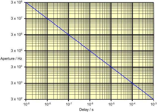
In many instances an aperture around Δf = 0.3 / τg,meas provides optimum measurement accuracy. For a measured group delay of 1 ns (corresponding to a cable with an electrical length of approx. 30 cm), this condition results in an aperture of 300 MHz. Optimum apertures for other group delay values are listed below. In the following example, the measured group delay is approx. 3 ns. A 100 MHz aperture virtually eliminates the noise on the trace.

The 100 MHz aperture in the example above is actually too wide, because the phase shows strong distortions in a frequency interval with a width of approx. 80 MHz. The wide aperture results in a smoothing effect of the delay trace. A reduced aperture of 20 MHz yields a more accurate group delay in the vicinity of the minimum.

The following table lists "optimum" apertures Δf = 0.3 / τg,meas together with sample analyzer settings for a frequency sweep with 201 sweep points. Notice that the sweep span must be reduced or the number of frequency points increased to obtain small apertures.

Group delay τg,meas	Aperture Δf	Span	No. of aperture steps
1 ns	300 MHz	6 GHz	10
10 ns	30 MHz	600 MHz	10
100 ns	3 MHz	60 MHz	10
1 μs	300 kHz	6 MHz	10
10 μs	30 kHz	600 kHz	10
10 μs	3 kHz	60 kHz	10
1 ms	300 Hz	6 kHz	10

The relationship between group delay and "optimum" aperture is also shown in the following diaram.

For more information about group and phase delay measurements refer to the application note 1EZ35_1E which is available for download on the Rohde & Schwarz internet.

http://www2.rohde-schwarz.com/en/products/test_and_measurement/network_analysis/?_view=downloads&downloadtype=20&type=20&downid=1550

SWR

Calculates the Standing Wave Ratio (SWR) from the measured quantity (primarily: from a reflection S-parameter) and displays it in a Cartesian diagram.

Properties: The SWR (or Voltage Standing Wave Ratio, VSWR) is a measure of the power reflected at the input of the DUT. It is calculated from the magnitude of the reflection coefficients Sii (where i denotes the port number of the DUT) according to:

The superposition of the incident and the reflected wave on the transmission line connecting the analyzer and the DUT causes an interference pattern with variable envelope voltage. The SWR is the ratio of the maximum voltage to the minimum envelope voltage along the line.

The superposition of the incident wave I and the reflected wave R on the transmission line connecting the analyzer and the DUT causes an interference pattern with variable envelope voltage. The SWR is the ratio of the maximum voltage to the minimum envelope voltage along the line:

SWR = VMax/VMin = (|VI| + |VR|) / (|VI| – |VR|) = (1 + |Sii|) / (1 – |Sii|)

Application: Reflection measurements with conversion of the complex S-parameter to a real SWR.

Lin Mag

Selects a Cartesian diagram with a linear vertical axis scale to display the magnitude of the measured quantity.

Application: Real measurement data (i.e. the Stability Factors, DC Input 1/2, and the PAE) are always displayed in a Lin Mag diagram.

The magnitude of each complex quantity can be displayed on a logarithmic scale. It is possible to view the real and imaginary parts instead of the magnitude and phase.

Real

Selects a Cartesian diagram to display the real part of a complex measured quantity.

Properties: The stimulus variable appears on the horizontal axis, scaled linearly. The real part Re(C) of the complex quantity C = Re(C) + j Im(C), appears on the vertical axis, also scaled linearly.

Application: The real part of an impedance corresponds to its resistive portion.

It is possible to view the magnitude and phase of a complex quantity instead of the real and imaginary part. The magnitude can be displayed on a linear scale or on a logarithmic scale. Both the real and imaginary parts are displayed in the polar diagram.

Imag

Selects a Cartesian diagram to display the imaginary part of a complex measured quantity.

Properties: The stimulus variable appears on the horizontal axis, scaled linearly. The imaginary part Im(C) of the complex quantity C = Re(C) + j Im(C), appears on the vertical axis, also scaled linearly.

Application: The imaginary part of an impedance corresponds to its reactive portion. Positive (negative) values represent inductive (capacitive) reactance.

Inverted Smith

Selects an inverted Smith chart to display a complex quantity, primarily a reflection S-parameter.

Properties: The Inverted Smith chart is a circular diagram obtained by mapping the positive complex semi-plane into a unit circle. If the measured quantity is a complex reflection coefficient (S11, S22 etc.), then the unit Inverted Smith chart represents the normalized admittance. In contrast to the polar diagram, the scaling of the diagram is not linear.

Unwrapped Phase

Selects a Cartesian diagram with an arbitrarily scaled linear vertical axis to display the phase of the measured quantity.

Properties: The stimulus variable appears on the horizontal axis, scaled linearly. The phase of the complex quantity C, i.e. φ (C) = arctan ( Im(C) / Re(C) ), appears on the vertical axis. φ (C) is measured relative to the phase at the start of the sweep (reference phase = 0°). In contrast to the normal Phase format, the display range is not limited to values between –180° and +180°. This avoids artificial jumps of the trace but can entail a relatively wide phase range if the sweep span is large.

Application: Phase measurements, e.g. phase distortion, deviation from linearity.

After changing to the Unwrapped Phase format, use Trace – Scale – Autoscale to re-scale the vertical axis and view the entire trace.