Opens a submenu to evaluate and display statistical and phase information of the entire trace or of a specific evaluation range and calculate the x-dB compression point.
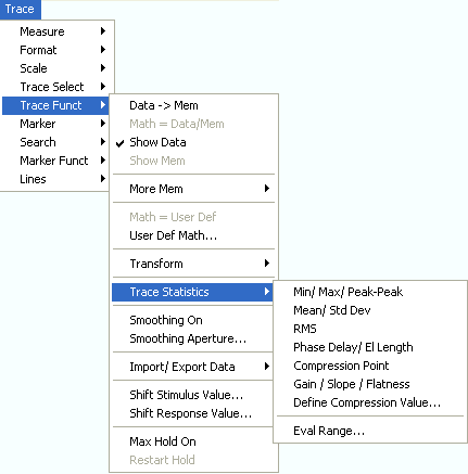
Min/Max/Peak-Peak displays or hides the essential statistical parameters of the trace in the selected evaluation range.
Mean/Std Dev displays or hides the arithmetic mean value and the standard deviation of the trace in the selected evaluation range.
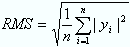
RMS displays or hides the RMS value of the trace in the selected evaluation range.
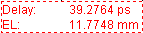
Phase Delay/El Length displays or hides the phase delay and the electrical length of the trace in the selected evaluation range (Eval Range...).
Compression Point starts the x-dB compression point evaluation
Define Compression Value... sets the compression level (x dB).
Gain/Slope/Flatness displays or hides trace parameters for the current evaluation range.
Eval Range... opens a dialog to define the range for the statistical and phase evaluation and for the compression point measurement.
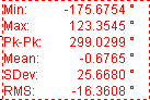
The first three commands in the Trace Statistics submenu display or hide the maximum (Max.), minimum (Min.), the peak-to-peak value (Pk-Pk), arithmetic mean value (Mean), the standard deviation (Std. Dev.), and the RMS value of all response values of the trace in the selected evaluation range (Eval Range...).
 Definition
of statistical quantities
Definition
of statistical quantities
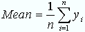
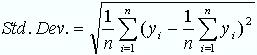
The statistical quantities are calculated from all response values in the selected evaluation range. Suppose that the trace in the evaluation range contains n stimulus values xi and n corresponding response values yi (measurement points).
Min. and Max. are the largest and the smallest of all response values yi.
Pk-Pk is the peak-to-peak value and is equal to the difference Max. – Min.
Mean is the arithmetic mean value of all response values:
SDev is the standard deviation of all response values:
RMS is the root mean square (effective value) of all response values:
 To calculate the Min.,
Max., Pk-Pk values and the SDev,
the analyzer uses formatted response values yi
(see trace formats).
Consequently, the mean value and the standard deviation of a trace depend
on the selected trace format.
To calculate the Min.,
Max., Pk-Pk values and the SDev,
the analyzer uses formatted response values yi
(see trace formats).
Consequently, the mean value and the standard deviation of a trace depend
on the selected trace format.
In contrast, the RMS calculation is based on linear, unformatted values.
The physical units for unformatted wave quantities is 1 Volt. The RMS
value has zero phase. The selected trace format is applied to the unformatted
RMS value, which means that the RMS result of a trace does depend on the
trace format.
Displays or hides the phase delay (Delay) and the electrical length (EL) of the trace in the selected evaluation range (Eval Range...). The parameters are only available for trace formats that contain phase information, i.e. for the formats Phase, Unwrapped Phase, and the polar diagram formats Polar, Smith, Inverted Smith. Moreover, the sweep type must be a frequency sweep.
Definition
of phase parameters
The phase parameters are obtained from an approximation to the derivative of the phase with respect to frequency in the selected evaluation range.
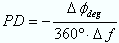
Delay is the phase delay, which is an approximation to the group delay and calculated as follows:
 ,
,
where Δf is the width of the evaluation range and DF is the corresponding phase change. See also note on transmission and reflection parameters below.
EL is the electrical length, which is the product of the phase delay times the speed of light in the vacuum.
If no dispersion occurs the phase delay is equal to the group delay. For more information see mathematical relations.
If a dispersive connector type (i.e. a waveguide; see Offset Modeldialog) is assigned to a test port related to a particular quantity, then the dispersion effects of the connector are taken into account for the calculation of the phase delay and the electrical length.
To account for the propagation in both directions,
the delay and the electrical length of a reflection parameter is only
half the delay and the electrical length of a transmission parameter.
The formula for PD above is for transmission parameters. See also introduction
to section Channel
– Offset.
The phase parameters are available only if
the evaluation range contains at least 3 measurement points.
 The phase evaluation can cause misleading
results if the evaluation range contains a
The phase evaluation can cause misleading
results if the evaluation range contains a  360 deg phase
jump. The trace format Unwrapped
Phase
avoids this behavior.
360 deg phase
jump. The trace format Unwrapped
Phase
avoids this behavior.
The
delay for reflection factors corresponds to the transmission time in one direction; see Offset –
Auto Length –
Length
and Delay Measurements.
|
Remote control: |
CALCulate<Chn>:STATistics[:STATe] |
Displays or hides all results related to the x-dB compression point of the trace, where x is the selected compression value. To obtain valid compression point results, a power sweep must be active, and the trace format must be dB Mag.
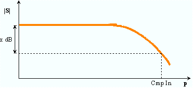
The x-dB compression point of an S-parameter or ratio is the stimulus signal level where the magnitude of the measured quantity has dropped by x dB compared to its value at small stimulus signal levels (small-signal value). As an approximation for the small-signal value, the analyzer uses the value at the start level of the evaluation range (Eval Range...).
The compression point is a measure for the upper edge of the linearity
range of a DUT. It is close to the highest input signal level for which
the DUT shows a linear response (|an|
—>
x*|an| ![]() |bn| —>
x*|bn|, so that the magnitude
of all S-parameters remains constant).
|bn| —>
x*|bn|, so that the magnitude
of all S-parameters remains constant).
When Compression Point is activated, a marker labeled Cmp is placed to compression point with the smallest stimulus level. Moreover the Trace Statistics info field shows the numerical results of the compression point measurement:
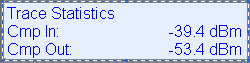
Cmp In is the stimulus level at the compression point in units of dBm. Cmp In always corresponds to the driving port level (e.g. the level from port no. j, if a transmission parameter Sij is measured).
Cmp
Out is the sum of the stimulus level Cmp
In and the magnitude of the measured response value at the compression
point.
The magnitude of a transmission S-parameter Sij
is a measure for the attenuation (or gain) of the DUT, hence: Cmp
Out = Cmp In + <Attenuation>. The example above is based
on an attenuation of –14
dB, hence Cmp Out = –39.4
dB –
14 dB = –53.4
dBm.
The info field shows invalid results ('---') if the wrong sweep type or trace format is selected, or if the trace contains no x-dB compression points in the selected evaluation range.
 Measuring
the x-dB compression point
Measuring
the x-dB compression point
|
Remote control: |
CALCulate:STATistics:NLINear:COMP[:STATe] |
Opens the numeric entry bar to define the compression value x (in dB) for the compression point measurement.
|
Remote control: |
Displays or hides trace parameters that the analyzer calculates for the current evaluation range. If no evaluation range is defined, the parameters apply to the sweep range.
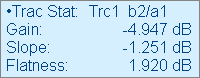
Suppose that A and B denote the trace points at the beginning and at the end of the evaluation range, respectively.
Gain is the larger of the two stimulus values of points A and B.
Slope is the difference of the stimulus values of point B minus point A.
Flatness is a measure of the deviation of the trace in the evaluation range from linearity. The analyzer calculates the difference trace between the active trace and the straight line between points A and B. The flatness is the difference between the largest and the smallest response value of this difference trace.
|
Remote control: |
CALCulate<Chn>:STATistics:SFLatness[:STATe] |
Opens a dialog to define the range for the statistical and phase evaluation and for the x-dB compression point measurement. The evaluation range is a continuous interval of the sweep variable.
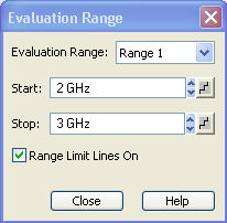
It is possible to select, define and display up to ten different evaluation ranges for each setup. Full Span means that the search range is equal to the sweep range. The statistical and phase evaluation and the compression point measurement take into account all measurement points with stimulus values xi between the Start and Stop value of the evaluation range:
Start  xi Stop
The evaluation ranges are identical to the
marker search ranges. For more information see Search
Range Dialog.
Activates the smoothing function for the active trace, which may be a data or a memory trace. With active smoothing function, each measurement point is replaced by the arithmetic mean value of all measurement points located in a symmetric interval centered on the stimulus value. The width of the smoothing interval is referred to as the Smoothing Aperture and can be adjusted according to the properties of the trace.
The sweep
average
is an alternative method of compensating for random effects on the trace
by averaging consecutive traces. Compared to smoothing, the sweep average
requires a longer measurement time but does not have the drawback of averaging
out quick variations of the measured values.
|
Remote control: |
Defines how many measurement points are averaged to smooth the trace if smoothing is switched on. The Smoothing Aperture is entered as a percentage of the total sweep span.
An aperture of n % means that the smoothing interval for each sweep point i with stimulus value xi is equal to [xi – span*n/200, xi + span*n/200], and that the result of i is replaced by the arithmetic mean value of all measurement points in this interval. The average is calculated for every measurement point. Smoothing does not significantly increase the measurement time.
 Finding
the appropriate aperture
Finding
the appropriate aperture
A large smoothing aperture enhances the smoothing effect but may also average out quick variations of the measured values and thus produce misleading results. To avoid errors, observe the following recommendations.
Start with a small aperture and increase it only as long as you are certain that the trace is still correctly reproduced.
As a general rule, the smoothing aperture should be small compared to the width of the observed structures (e.g. the resonance peaks of a filter). If necessary, restrict the sweep range or switch smoothing off to analyze narrow structures.
|
Remote control: |
